Classification Models on Satellite Images
Data
I analyzed the SAT-4 Airborne Dataset provided by the National Agriculture Imagery Program and compiled by the Bay Area Environmental Research Institute/NASA Ames Research Center.
The dataset consists of 500,000 satellite images of the Earth’s surface. Each image is 28x28 pixels large. The images are in color and also include near infrared information. Therefore, the observed data is a 28x28x4x400000 array of uint8 variables (that is, integers between 0 and 255). The last dimension encodes the index of the image. The first and second dimensions encode the row and column, respectively, of the pixel. The third dimension describes the channel: index 0 is red, 1 is green, 2 is blue, and 3 is NIR.The variable train y provides the labels for the training set.
Summary
In order to build a classifier that labels satellite images into one of four labels: “barren land”, “trees”, “grassland”, or “none”, I optimized three different types of models being SVM, Logistic Regression using PyTorch, and Gradient Descent. After training and validating each model, SVM was shown to have the best performance model. Since the model choice was SVM, I further fit this onto an outside sample dataset with the previously selected parameters using the pickle module. To test this, visit my github for my files! The model.dat file can be generated by running the train.ipynb file. The satellite.ipynb reads the model.dat and returns a file named “landuse.csv” that should contain all of the classifier predictions.
Data Preprocessing
Since the data is very complex with having my dimensions per image, I decided to compile the original four channels for each image into one channel, making the images in a grayscale. I have also split my training dataset even further to have a validation set that is of .1 the size of the training dataset.
Modeling
Classifier 1: Logistic Regression with PyTorch
Using the transformed grayscale dataset, I transformed the dataset to a tensor form and concatenated it with the labeled data. Next, I randomly picked 20% of the images for the validation set and randomly took a subset of each validation and training of size 100. Before feeding the resulting batch to the logistic regression model, I flattened each image tensor to a vector of size 784. The output for each image is a vector size of 4, with each element of the vector signifying the probability of a particular label. The predicted label for an image is the one with the highest probability.
I ran the resulting batch through the logistic regression model. By choosing the index of the element with the highest probability in each output row, I ran through the classifier of the prepared data. Next, I evaluated the metric and loss function to see how well the model is performing. To do this, I found the percentage of labels that were predicted correctly and this accuracy ends up being 40%. I have also used the cross entropy that is built into PyTorch. Unlike the accuracy metric I used prior, cross entropy is a continuous and differentiable function which makes it a good choice for a loss function.
I conducted parameter selection by running the model the model with various parameters in learning rate and batch size. The success metrics tied to the parameters are shown in the table below. I chose the optimal learning rate to be .05 since it gave a slightly higher accuracy for the correct label, indicating a lower loss metric when I fitted the model over multiple epochs.
Parameter selection for different learning rates
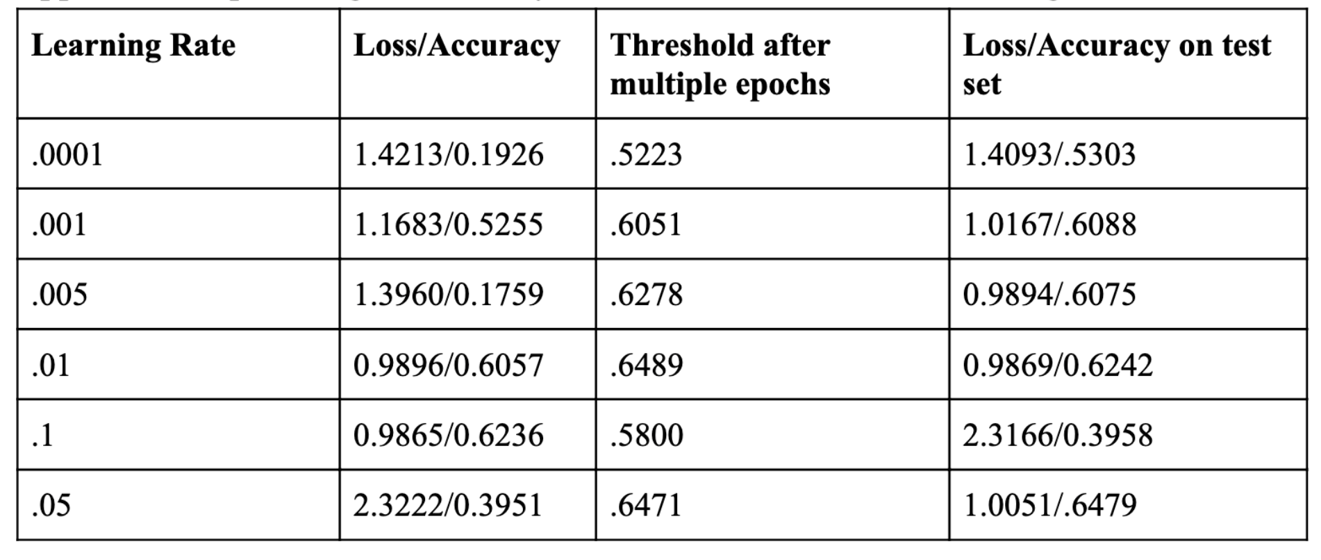
In training the data, I built functions that would calculate the loss for a batch of data and the overall loss of the validation data. On the validation data, I got a 61% accuracy and a loss of 1.01. The accuracy is satisfactory since the accuracy is greater than 25%– which is the chance that the model would correctly classify a label by randomly guessing. In terms of neural networks, an epoch refers to one cycle through the full training dataset. In order to optimize the model, I have trained the data for more than one epoch, hoping for a better generalization when given a new set of batch data. In total, I trained about 18 epochs.
Accuracy of the Logistic Regression Model over various numbers of epochs**
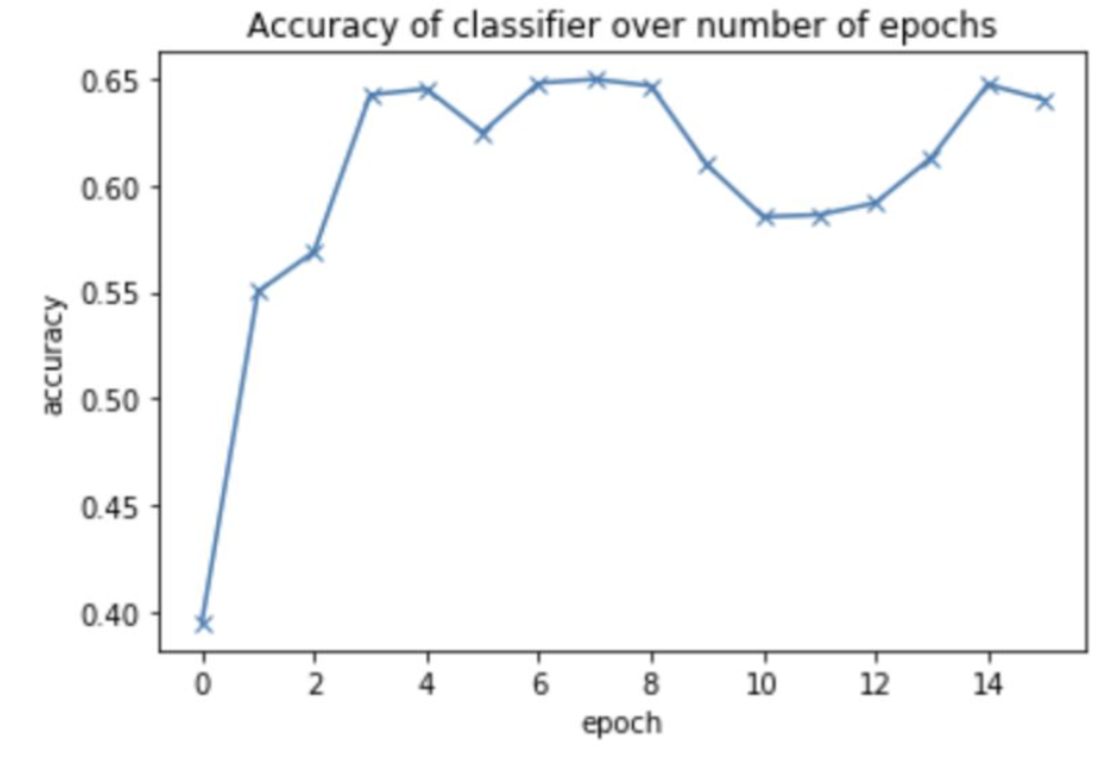
The line graph shows that there are improvements after every epoch up until a certain threshold where it plateaus. The model won’t cross the threshold of 61% even after training for a long time. And for evaluating the model performance on the test data, I also obtained an accuracy of 61%. One possible reason for this is that the learning rate might be too high. It’s possible that the model’s parameters miss the optimal set of parameters that have the lowest loss. For further investigation, I can reduce the learning rate and training for a few more epochs to see if it helps. The model may not have been as powerful as the SVM model because I have assumed that the result (probabilities) is a linear function of the pixel features from doing a matrix multiplication with the weight matrix and adding bias. However, there may not be a linear relationship between the two.
Classifier 2: Support Vector Machine
Unoptimized SVM
I ran a preliminary model with the split training set through the sklearn.svm package and a kernel-based SVM. Then I had used the params from the training dataset to predict the labels from the test set. The accuracy of the model with the test set came out to be 83%. I have found the accuracy to be satisfactory but this model took very long to run. Therefore, I would like to try using the linear SVM which would be much faster and could scale a lot better.
Classification report for SVM classification model (kernel based SVM)

Optimized SVM
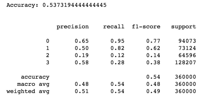
With the linear kernel, I actually obtained a lower accuracy on the test set of around 54%.
Classification report for SVM classification model (linear based SVM)
In the process of further optimizing the support vector machine, I noticed that one of the disadvantages of support vector machines is that they are not scale invariant; therefore, I made the decision to normalize each feature to be between 0 and 1 before training the classifier. Next, I flattened the four-dimensional array into a one-dimensional array of features. With the flattened features array, I looped over all 400,000 images to create features for each image and stacked the flattened features into a big feature matrix. The resulting feature matrix is shaped so that the rows represent the images and the columns contain the features with 400,000 images and 784 features. The training dataset has now the shape of (360000,784). To avoid overfitting, I wanted to reduce the size of the features by linearly transforming the data so that most of the information in the data is contained within a small number of components. I did this by using sklearn’s PCA built in function.
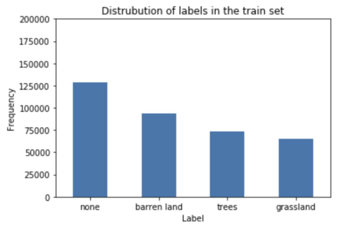
Before training the model, I plotted the distribution of labels in the train set that’s shown below. Based on the plot, there is a slightly more instances of “none” images compared to the rest of the type of images. Though “none” had the most instances, the overall distribution across the labels don’t seem too unbalanced.
Distribution of labels in the training set
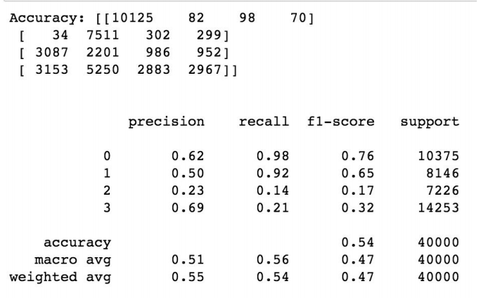
Along with accuracy, I observed the Confusion Matrix–which is a breakdown of predictions into a table showing correct predictions and the types of correct predictions made. After running through the data through the SVM linear kernel, the model accuracy on the test set is .55 for weighted average. For more details on the performance of the model.
Classification report for the SVM Classification Model (Linear Kernel) with normalized and feature transformed dataset
Classifier 3: Stochastic Gradient Descent
Initial model for Stochastic Gradient Descent
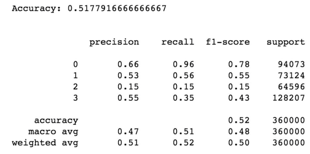
Stochastic Gradient Descent is a simple yet very efficient approach to learning linear classifiers under convex functions such as the linear SVM and Logistic Regression, the two models that I ran prior. The Stochastic Gradient Descent is advantageous since it is efficient. The accuracy of the model when used on the test set was around .52, more details in the performance of the model given in the report below.
Classification report for the Stochastic Gradient Descent Model
Optimize Stochastic Gradient Descent
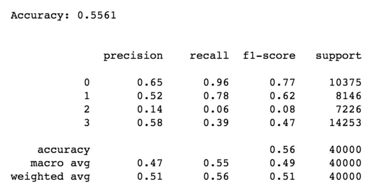
By using sklearn’s PCA built in function, the accuracy has increased but not significantly. The accuracy obtained is around .56 with more details shown in the report below.
Classification report for the Optimized Stochastic Gradient Descent Model
Conclusion
In conclusion, I have decided to use the model with the highest accuracy. Surprisingly this came out to be the SVM classification model that is kernel based. The reason why this may be the strongest model that I have built is because the output in classification may not be linear with the input (the pixel features of the images).
References
- S, Aakash N. “Image Classification Using Logistic Regression in PyTorch.” Medium, DataScienceNetwork(DSNet),13May2019, medium.com/dsnet/image-classification-using-logistic-regression-in-pytorch-ebb96cc9eb 79.
- Galarnyk, Michael. “PCA Using Python (Scikit-Learn).” Medium, Towards Data Science, 4 Nov. 2019, towardsdatascience.com/pca-using-python-scikit-learn-e653f8989e60.
- Galarnyk, Michael. “PCA Using Python (Scikit-Learn).” Medium, Towards Data Science, 4 Nov. 2019, towardsdatascience.com/pca-using-python-scikit-learn-e653f8989e60.
- “1.4. Support Vector Machines.” Scikit, scikit-learn.org/stable/modules/svm.html.