Predicting Wine Ratings
Summary
Wine ratings is an important issue as it affects both the sellers and the buyers. For the buyers, wine ratings can help the buyers with their decision in buying a wine by providing insight of expectations on how the wine should taste through tasting notes and the score. As for the sellers, wine ratings can help promote their brand and their product in the market to grow their business. Knowing the characteristics that make a high-rating wine can also help sellers aim for higher ratings in their next manufacturing cyce, and buyers would also have more insight in choosing good quality wines.
Overall, I was able to find that wine characteristics have different predictive power as well as different effects (negative/positive) on wine ratings, depending on whether the wine is white or red. I also found that residual sugar, wine color, chlories, total sulfur dioxide, sulphates, alcohol, and rating all had statistically significant relationships with wine rating proved by the t-test hypothesis testing. However, I was unable to prove that density and pH had a significant relationship with wine rating. Using all the wine characteristics combined, I was able to make a sufficient prediction in wine ratings. With a majority of high predictive wine characteristics, the multinomial logistic regression model was able to predict wine ratings with a 52% accuracy rate while the modified and improved logistic regression model predicted wine quality with a 70% accuracy rate.
To look at the code in more detail, check out my github repo
Data
I analyzed the dataset provided by Paulo Cortez, an Associate Professor at the University of Minho, along with several other individuals (António Cerdeira, Fernando Almeida, Telmo Matos, José Reis) and the Viticulture Commission of the Vinho Verde Region.
There are 6497 total instances in this dataset. Each instance represents a wine and it’s properties, which are its physiochemical qualities and its rating. There is only one type of instance here.
Data Preprocessing
The data was already very preprocessed when I sourced it from the machine learning repository. Checking the data types of the columns, they’re pretty much all floats, which means that the data was already cleaned up by the University or someone else when I downloaded it. I dropped some columns since they seemed to imply the same thing, such as acidity levels, as well as because there are already so many columns already. The datasets were combined as well, into one large dataframe so analysis could be done over the entire dataset as a whole.
Preregistration Statement
I will aim to pinpoint the most important feature(s) that are most important in assessing the quality of wine. I will delve into this matter by observing the correlation between these features and the predictor variable, rating. In the follow up analysis, I would also like to see whether the significant features for wine rating differ between red and white wine. After gaining an insight on how significant the provided wine characteristics are for wine rating, I hope to predict wine rating with a logistic regression model. To aim for a good model performance, I will also try to optimize the model so that it generalizes well (meaning it won’t underfit or overfit) and has a reasonable accuracy rate. These regression models will provide further information to anayze the feature importance further with the features’ coefficients and the model score to see how much of the variability in wine rating is explained by the features.
Also, it’s important to note that in a real world application that wines are generally tasted blind, so the taster doesn’t have any information about the wine except for the general grape varietal (Chardonnay, Cabernet, etc) and the vintage. Therefore, the taster is able to deduce whether the tasted wine is red or white based on the grape varietal. This research will provide an insight on whether there are certain wine characteristics that were already predetermined in the wine community that make a good white wine and red wine through the feature importance analysis. By developing a highly accurate model, I could potentially use data science to rate wine, diminishing the possibility of human bias and error that occurs during the wine rating process as the rating can be subjective to a certain extent. Because wine rating affects both wine producers’ (making or breaking their business) and buyers (assisting their shopping choices), this research aims to analyze wine quality patterns and predict wine rating with a high accuracy rate.
Data Analysis
A preview of the first five rows and all the included columns of the dataset:

Exploratory Data Analysis
To start off the exploratory data analysis, I want to look at the distribution of values in the rating’s column, as well as look at the medium and median for the wine ratings. I use a histogram to do so.
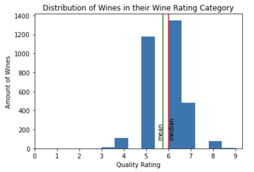
This historam shows that the distribution of the wines in the dataset are centered aorund 6. The histogram is also slighly negatively skewed with the median rating being larger than the mean rating. It is worth noting that more of the wines are based on higher ratings with the lower rating wines are pulling the mean lower in value.
Since the overwhelming majority of these wines are centered around 6, I isolated the top 2 and bottom 2 ratings into their own dataframes to gain more insight about the lowest rated wines and the highest rated wines.
top_wines = wine[wine['rating'] >= 8].copy()
bottom_wines = wine[wine['rating'] <= 4].copy()
Next, I am going to look at the means and medians of all columns for high rated wines. However, this was quite hard to read concisely, so instead, I’m going to look at the difference between the top_wines means and all wines means in each column, and do the same for the bottom_wines means and all wines means.
col_names = wine.columns
col_names.drop('rating')
print("Differences in wine column means from top wines to all wines")
print(top_wines[col_names.drop('rating')].mean().subtract(wine[col_names.drop('rating')].mean()))
print("Differences in wine column means from all wines to bottom wines")
print(wine[col_names.drop('rating')].mean().subtract(bottom_wines[col_names.drop('rating')].mean()))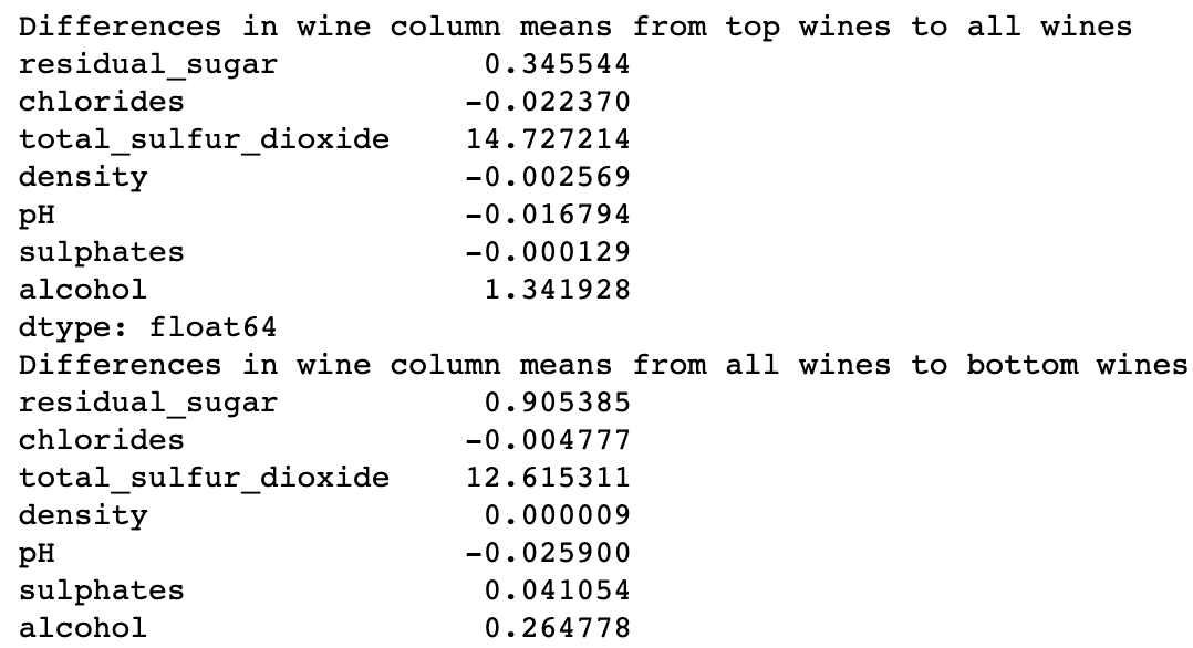
When taking the difference in means for each feature between all wines to bottom wines, there’s not much of a change in anything other than mean total_sulfur_dioxide, and mean residual_sugar. On the other hand, when taking the difference in means for each feature between all wines to top wines, the only significant differences of means are for the total_sulfur_dioxide and alcohol features.
However, the wine characteristics in the data are currently under different units, so it’s not enough to just pick the highest numbers, but I also want to see if these differences portray a large change in the unit of that column by using the boxcharts below. I would like to investigate whether the three “significant” features that were mentioned above actually have considerably large differences based on the distribution of values given by the following box-plots. For example, if alcohol has an interquartile range from 1-100 in the data, it’s change of 1.3 won’t mean much as a change of 1.3 would describe a small portion of existing values.
Looking more into the total_sulfur_dioxide, residual_sugar, and alcohol, I chart out box-plots for each of them.
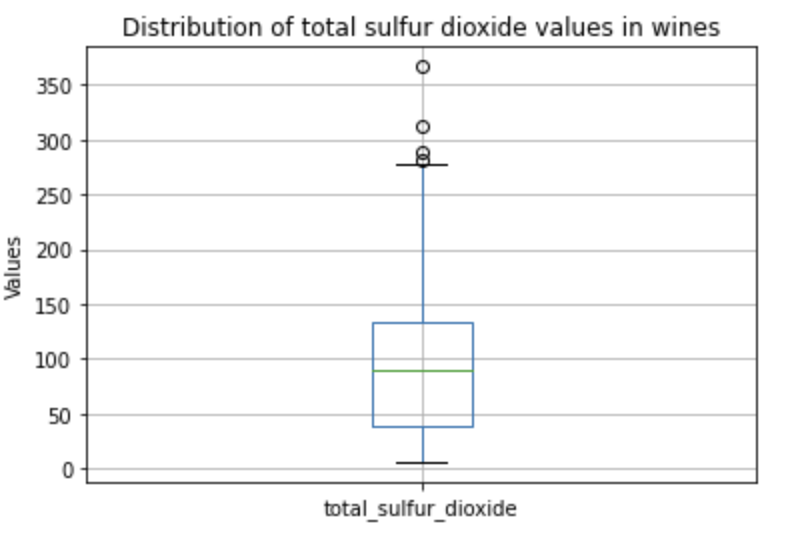
In this boxplot for the total sulfur dioxide the box does not seem to be squished and there is a moderate amount of outliers out of the boxplot and these points are not too far off.
I then look at the interquartile values, which range from 45 to 135. I choose to use these because this range represents 50% of the data, and helps us avoid taking into account outliers and data that might be too skewed in one direction or the other.
As the interquartile values range from 45 to 135, so the values of 12.62 and 14.73 give us about 16.3% (which I got from 14.73 / (135 - 45) ) of the interquartile range. A change of that magnitude in the sulfur dioxide between the ‘good’ and ‘average’ wines isn’t extremely large, but isn’t something I should entirely ignore either.
From here, I see that the change in total_sulfur_dioxide from top wines to all wines isn’t really much of a change when looking at the total scale of values.
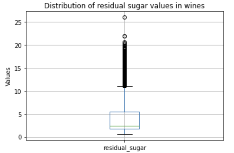
The mean differences for residual sugar were 0.35 and .91, which on an interquartile range of 2-6, indicates a change of about 8.5% and 22.7% for top and bottom wines respectively in the residual sugar level. As such, the mean difference for residual sugar likely doesn’t mean much for differentiating between top and average wines, but might mean more for differentiating beween average and bottom wines.
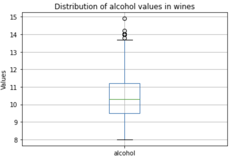
Alcohol has a 1.34 and 0.26 mean differences for top wines to average wines and average wines to bottom wines respectively. When I look at the boxplot, the interquartile values range from 9.5 to 11.2. This gives us a change of 79% and 15% for top wines to average wines and average wines to bottom wines respectively. As such, alcohol is likely a bigger factor in differentiating between top wines and average wines, but a smaller factor for differentiating between average wines and bottom wines.
So out of the three attributes I picked, it seems that alcohol has a large difference in it’s mean between top wines and average wines, residual sugar has a large difference in means between bottom wines and average wines, and total sulfur dioxide is equally different in differentiating top wines from average wines and bottom wines from average wines.
Next, I’ll try to plot these relationships between rating and the three attributes I just went through on a scatter plot
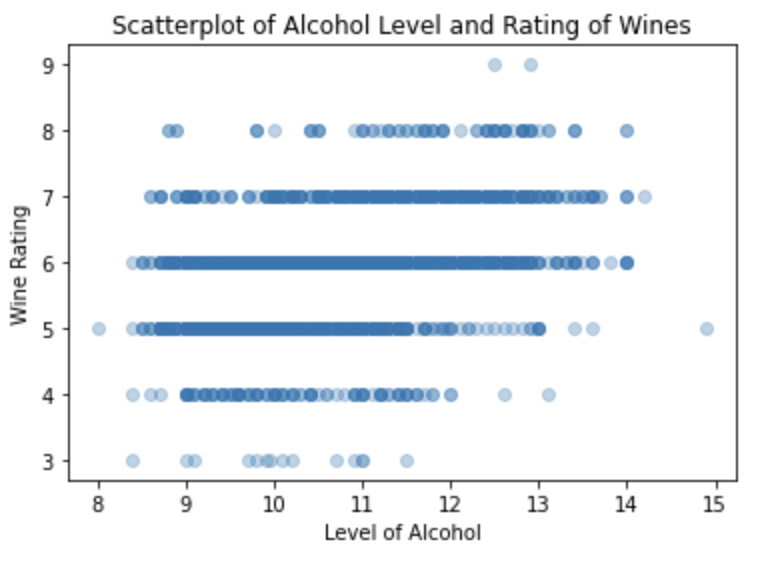
I see that the distribution of wine ratings across levels of alcohol can arguably be uniform. For example, wines that are rated as a 7, there is a uniformity across these wines that range from 10 to 13 levels of alcohol. There isn’t as much data for wines that are rated 8 and above as well as 4 and below. It seems that I can make the best deductions with the wines that are rated between 5-7 as there is enough observations in the dataset. Similarly to the wines rated as 7, the wines rated as 6 has mostly a uniform distribution across 9-13 levels of alchol and wines rated as 5 uniformly contains 8.5-12 range of alcohol levels. Though these wine rating categories exhibit close to uniform distributions across levels of alcohol, the parameters for the uniform distributions differ as shown in the varying ranges for each wine rating category. The varying parameters can signify that alcohol levels can play a large plot in predicting wine rating.
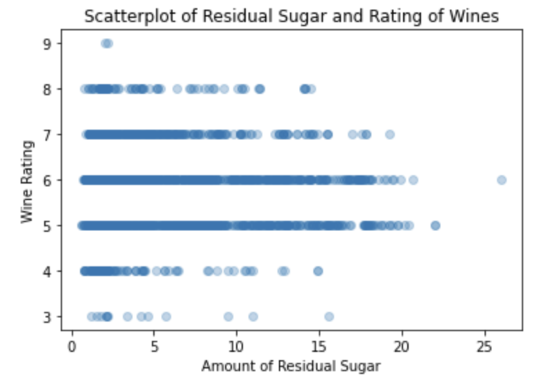
From the same reasoning as the first scatterplot, I will exclusive observe wines that were rated between 5-7 for the sake of having enough information in the dataset. I see uniformity of distribution across residual sugar for wines rated as 5 and 6 with ranges 0-17 and ranges 0-18 respectively. I see that wines rated as 7 has a more sparse distribution towards the higher values for residual sugar signifying a possible right skewed distribution, meaning that more of the wines rated as 7 tend to be around the lower levels of residual sugar.
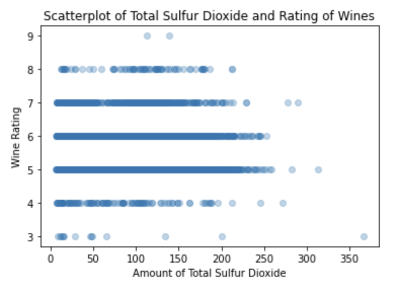
From the same reasoning as the firs two scatterplots, I will exclusive observe wines that were rated between 5-7 for the sake of having enough information in the dataset. I see uniformity of distribution across total sulfur dioxide for wines rated as 5,6, and 7 with range 0-250, range 0-250, and range 0-225 respectively. Compared to the first scatterplot with alcohol levels, I see that all the different wine ratings have uniform distribution with total sulfur dioxide but arguably has similar parameters/ranges for the uniform distribution. I can deduce from this plot that there is at least, slight hints, if any, of influence of total sulfur dioxide on wine rating.
Overall, the distributions largely seem uniform, with alcohol being the one that I could see a little bit of positive correlation for. On that note, it seems to be good for us to look at correlation matrix now among all columns.
Feature Importance Analysis
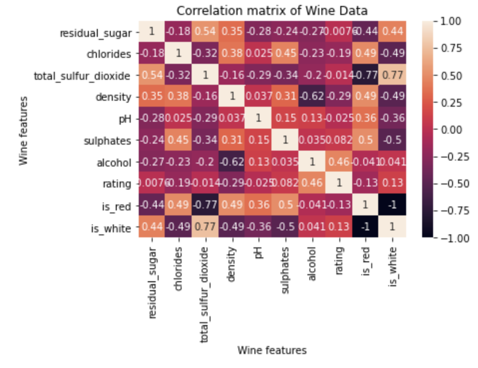
Interestingly, if the wine is red, the rating would decrease by 0.13 and if the wine is white, the rating would increase by 0.13. I see that the wine characteristics, generally, that make a high-rating wine are that it is a white wine, higher alcohol, higher sulphates, lower pH, lower density, lower total sulfur dioxide, lower chlorides, and lower residual sugar. The wine characteristics that have more predictive power, meaning more of a magnitudinal value (from greatest to least) are alcohol, density, chlorides, and wine color. Though there were very low correlations in variables like residual sugar, total sulfur dioxide, pH, and sulphates, fortunately, there were variables such as chlorides, density, alcohol, and wine color that had a correlation with wine rating that was at least .1 in magnitude. With at least 4 influential features, it seems to be somewhat promising to achieve a reasonable accuracy rate when predicting wine rating.
total_wine_mean = wine.rating.mean()
print("Mean of all wine ratings: {0:.3f}".format(total_wine_mean))
white_mean = wine.query("wine_color == 'white'").rating.mean()
print("Mean of White wine ratings: {0:.3f}".format(white_mean))
red_mean = wine.query("wine_color == 'red'").rating.mean()
print("Mean of Red wine ratings: {0:.3f}".format(red_mean))
#=> Mean of all wine ratings: 5.749
##  Mean of White wine ratings: 5.861
##  Mean of Red wine ratings: 5.636

print("{} observations for red wine".format(len(wine.query("wine_color == 'red'"))))
print("{} observations for white wine".format(len(wine.query("wine_color == 'white'"))))

#=> 1599 observations for red wine
##  1616 observations for white wine
Even though the number of observations for white wine and red wine are fairly balanced, there is still a difference in the average wine ratings for red and white wine, with white wine being .225 ratings greater than red wine. This could explain why the white color had a more positive correlation with wine rating while red color had a more negative correlation.
Signature Features for red and white wine
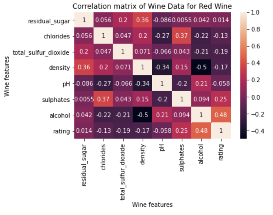
With red wine specifically, the most influential factors are alcohol, sulphates, and three other features that have similar correlations with rating: total sulfur dioxide, density, and chlorides. This differs from the general wine rating because sulphates and total sulfur dioxide greatly increased in magnitude.
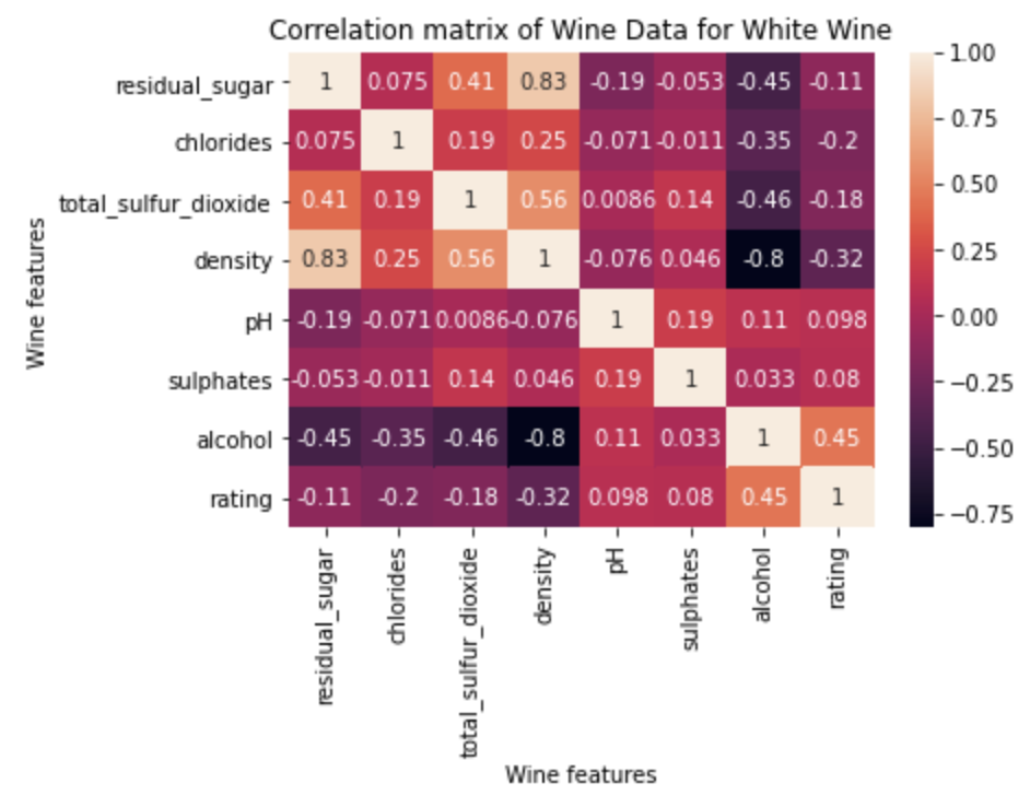
Looking at white wine specifically, I see that the most influential factors are alcohol, density, chlorides, residual sugar, and total sulfur dioxide. This differs from the general wine rating because total sulfur dioxide and residual sugar have greatly increased in magnitude.
Comparing the correlations of wine characteristics in red and white wine ratings gives us an insight that not only is there a difference in predictive power of wine features between red and white wine but these wine features could also have different effects (negative or beneficial) between the two types of wines.
- For residual sugar, an increment of one could increase the rating of red wine by 0.014 while dropping the white wine rating by 0.1.
- In this case, the effect is opposite on the ratings for red and white wine and having more of an impact on the white wine.
- For chlorides, an increment of one could drop the rating of red wine by 0.13 while dropping the white wine rating by 0.2.
- In this case, the effect is a similar direction on the ratings for red and white wine and having more of an impact on the white wine.
- For total sulfur dioxide, an increment of one could drop the rating of red wine by 0.19 while dropping the white wine rating by 0.18.
- In this case, the effect is in the same direction on the ratings for red and white wine and having slightly more of an impact on the red wine.
- For density, an increment of one could drop the rating of red wine by 0.17 while dropping the white wine rating by 0.32.
- In this case, the effect is in the same direction on the ratings for red and white wine and having more of an impact on the white wine.
- For pH, an increment of one could drop the rating of red wine by 0.058 while increasing the white wine rating by 0.098.
- In this case, the effect is opposite on the ratings for red and white wine and having more of an impact on the white wine.
- For sulphates, an increment of one could increase the rating of red wine by 0.25 while increasing the white wine rating by 0.08.
- In this case, the effect is the same direction on the ratings for red and white wine and having more of an impact on the red wine.
- For alcohol, an increment of one could increase the rating of red wine by 0.48 while increasing the white wine rating by 0.45.
- In this case, the effect is in the same direction on the ratings for red and white wine and slightly having more of an impact on the red wine.
So far, I see that the effect of wine characteristics on the wine quality differs when I analyze the wine dataset by wine color.
Predicting Wine Rating
Multinomial Logistic Regression
Before modelling, my data had to be standardized so that the distribution of each feature has a mean of 0 and standard deviation of 1 with a StandardScaler(). The data was also split into training and validation sets (80/20). Now, I am ready to fit the model:
#https://towardsdatascience.com/comparing-classification-models-for-wine-quality-prediction-6c5f26669a4f
from sklearn.metrics import accuracy_score
logreg = LogisticRegression(multi_class='multinomial',solver ='newton-cg')
logreg.fit(X_train, y_train)

# Predict out-of-sample test set
y_pred = logreg.predict(X_test)

# Print classification report
print(metrics.classification_report(y_test, y_pred, zero_division = 1))
print("Accuracy Rate of Multinomial Logistic Regression Model:",accuracy_score(y_test, y_pred))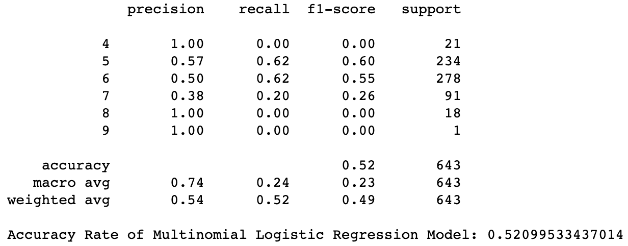
The classification report shows that classes 4,8, and 9 have not been taken into consideration when training because their recall results are zero and these classes have small numbers of observations available (with 21,18, and 1 observations respectively). This happens as there is an imbalance of wine observations that fall under the higher and lower rating classes and the model wasn’t able to get enough insight on wines with more extreme ratings during the training phase. This means that the model isn’t able to predict the wines in class 4,8,9 correctly. Furthermore, the accuracy rate for correct rating predictions was around 52%. This is arguably better than building a model that randomly classifies the rating out of 6 classes, which would have an accuracy rate of around 17%. However, because of the imbalance of data, I will improve the model even further by clustering the more extreme wines together and by creating broader categories. This way, the model will better recognize the wine characteristics that define a lower rated wine, and a higher rated wine.
Optimized Logistic Regression
Since the mean and median rating is centered around 6, any rating below 6 will be labelled as below average. For the sake of balancing the number of observations in each class, I did not want to leave 6 to be as its own class as it will cause the higher rated class to be deficient in observations. Therefore, a rating 6 and above is considered above average in the logistic regression model.
## Perform the regression
model = LogisticRegression().fit(X_train, y_train)
y_pred = model.predict(X_test)
# Print regression coefficients
coeff_df = pd.DataFrame(model.coef_,columns=X_features)
coeff_df
Since the data has been normalized and that all the features are under the same scale, I can confidently claim that from the magnitude of the regression coefficients that is at least greater than 0.2, alcohol, wine color, sulphates, total sulfur dioxide, residual sugar, and chlorides have great influential power in predicting wine rating. Density and pH seem to not have much of an influence in swaying the rating of the wine that’s predicted by the model.
# calculating the training and testing accuracies
print("Training accuracy :", model.score(X_train, y_train))
print("Testing accuracy :", model.score(X_test, y_test))
#=> Training accuracy : 0.7142301710730948
##  Testing accuracy : 0.6905132192846034
The training and testing accuracy were very similar to each other proving that I see a pretty good generalization happening with this model in that there is no overfitting taking place. Therefore, there is no need to reduce overfitting by reducing the complexity of the model by removing features. Even if I were to only include the most important features in predicting wine rating for all types of wine into this model, the variance of the model would not reduce too much. Instead, I should focus on increasing the bias of the model to increase the accuracy, which is currently around 70%, indicating that the logistic model was able to use all the given wine characteristics to properly label a wine as poor or top rated 70% of the time.
Further insight on feature importance using regression models that predict wine rating specifcally for white and red wine
Now, that I have built a model for predicting wine ratings on all wines, I want to build a similar logistic regression model but specifically on red wines, and then once again specifically on white wines.
Red wine

# calculating the training and testing accuracies
print("Training accuracy :", model.score(X_train, y_train))
print("Testing accuracy :", model.score(X_test, y_test))
#=> Training accuracy : 0.7357310398749023
##  Testing accuracy : 0.725
The most influential features with higher magnitudinal coefficients in the logistic regression model for red wines from greatest to least are alcohol, sulphates, total sulfur dioxide, chlorides, pH, and residual sugar. This is consistent with what I found earlier with the correlations as pH and residual sugar had the lowest correlations in magnitude out of all the other wine characteristics. The specific logistic regression model seemed to also have a good accuracy rate of around 72% and seems to be similar whether the model predicts in sample or out of sample.
White wine

# calculating the training and testing accuracies
print("Training accuracy :", model.score(X_train, y_train))
print("Testing accuracy :", model.score(X_test, y_test))
#=> Training accuracy : 0.7097523219814241
##  Testing accuracy : 0.6851851851851852
The most influential features with higher magnitudinal coefficients in the logistic regression model for white wines from greatest to least are alcohol, residual sugar, density, sulphates, pH, and chlorides. This seems to also agree with the results I found in the earlier correlation table for white wines when chlorides, pH, sulphates, and total sulfur dioxide were the features with lower correlations with wine rating in magnitude. The specific logistic regression model seemed to also have a good accuracy rate of around 70% and seems to be similar whether the model predicts in sample or out of sample.
The coefficients of the red wine logistic regression model change drastically compared to the coefficients of the white wine logistic regression model. Clearly, the magnitude of the coefficients of the wine characteristics changed. For example, total sulfur dioxide for white wine had a low coefficient of 0.08 while it had a coefficient of .49 for red white, a significant increase. Moreover, thought the wine characteristics primarily seemed to have the same direction (positive or negative) effect on wine rating, there was a conflict with pH. Since lower rated wines is indicated by 1 in this model, the negative coefficient for pH in white wine indicates that higher rated white wines have higher pH, while the positive coefficient for pH in red wine indicates that higher rated red wines have lower pH.
When predicting the ratings of white and red wine separately, the accuracies did not change much which makes sense because the original model had dummy variables to account for the wine type when predicting the wine rating already. It is pointless to compare the coefficients of the specific wine type logistic model because the coefficients would obviously be different to the general model, as the wine color feature gets taken away. Since a feature is removed, the coefficients of the other features would fluctuate and change.
Evaluation of Significance
#https://investigate.ai/regression/evaluating-logistic-regressions/
import statsmodels.formula.api as smf
sm_model= smf.logit("rating ~ residual_sugar + chlorides + total_sulfur_dioxide + density + pH + sulphates + alcohol + is_red",data=wine)
result = sm_model.fit()
result.summary()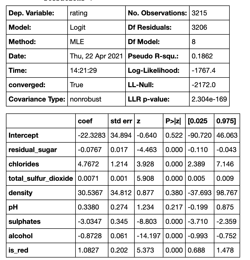
Looking at the p-values in the t-test, all of the wine characteristics have a very low p-value except for density, and pH. The p-value indicates the portion of samples that are outer in the tail area or samples that are greater than or equal to the corresponding t statistic value assuming that the null hypothesis is true. In this case, the null hypothesis is that there is no relationship between the wine characteristics and the wine ratings. This can be seen as the t-test aims to approximate large number of permutation tests where in each permutation test, the output has been shuffled and put together with the normal inputs to introduce randomness. This way, there is no relationship between the inputs and the outputs, thus being the null hypothesis. With a histogram of slopes from the permutation tests, I can use the p-value to indicate the portion of samples that are outer in the tail area or samples that are greater than or equal to the corresponding t statistic value assuming that the null hypothesis is true. Using a .05 significance level as a standard threshold, I can say that since all the p-values for all the wine characteristics are less than 0.05, I reject the null hypothesis that there is no relationship between these wine characteristics with the wine ratings. I reject the null hypothesis because there is a low probability of these samples occurring under the null hypothesis so I reject the null hypothesis. Even the wine colors have a relationship with the wine ratings as well. However, since the pvalues for density and pH is greater than 0.05, I fail to reject the null hypothesis for these characteristics, concluding that there is no relationship between pH and wine rating and no relationship between density and wine rating.
Interpretations and Conclusions
The research has found that wine characteristics have different predictive power and solemnly different effects (negative or positive) on wine ratings depending on whether the wine is white or red.
I did this by looking at the correlation coefficients of the wine characteristics with the wine rating separately for red and white wines. For both red and white wines, density, alcohol, chlorides had larger correlation coefficients, also having proven to have a statisically significant relationship with wine rating through a t-test. However, for red wine uniquely, sulphates had a large correlation coefficient of -0.690367 while white wine had a coefficient of -0.215922. Though this correlation analysis happened before normalizing the features in my data, there were little to none disparities in the results compared to the feature coefficients in the logistic regression model and to the results in my significance evaluation testing. The deductions for feature importance were fairly consistent in supporting the argument that all the provided wine characteristics, including wine color, and except density and pH have a relationship with wine rating. To answer the question on which wine characteristics would generally produce a better wine (bear in mind that a positive prediction in the logistic regression model indicates a low rated wine), I have found that higher alcohol, higher sulphates, higher residual sugar, lower total sulfur dioxide, and being white wine increase the quality of wine.
I am confident with this conclusion because the coefficients from the multivariable linear regression indicate the negative or positive influence on the wine rating, which is also backed by a t-test hypothesis testing. The very low LLR p-value (2.304e-169) indicated by the t-test hypothesis testing gave reason to believe that the logistic regression model, with a reasonable accuracy rate for training and testing data and statistically significant features that were proven to have a relationship with wine rating, could be trusted to predict wine ratings. For example, one of the wine characteristics, wine color, does have an effect on the wine rating, as initially indicated in the output of mean ratings for red and white wine. White wine was around .225 rating scores higher than red wine on average. This difference was proven to be significant with the t-test as the wine colors had a very low p-value, allowing me to reject the null hypothesis that there is no relationship between wine color and wine rating. Moreover, the coefficients for is_red_wine had a .55 (with 1 indicating lowly rated wine in the model), meaning that if the wine was white then the rating would increase by .55 and if red, the rating would drop by .55. Backed up by the t-test, the non-zero significance coefficient values were not due to randomness but that there was actually a relationship. This significance in relationship has been the case for other wine characteristics such as residual sugar, chlorides, total sulfur dioxide, sulphates, and alcohol. In addition, density and pH were not very significant in predicting wine rating as they had very high p-values in the t-test which meant that the nonzero coefficient values of 0.00829 and 0.08668 correspondingly for density and pH in the multivariable regression were due to random chance and there wasn’t significant proof to reject the hypothesis that there is no relationship between these two factors and wine rating.
By handling the imbalance of data across different wine rating categories, the logistic regression model was able to classify top rated and bottom rated wines reasonably well with an accuracy rate close to 70%. This is better than randomly guessing whether a wine is either top rated or bottom rated since the accuracy rate exceeds a 50% rate. Not only am I satisfied with the accuracy of the classifier, I am also satisfied with the fact that the model generalizes pretty well as shown by the close similarity between the training and testing accuracy rate.
Limitations
I have defined what characteristics would be good for red and white wine seperately but it could also be worthwhile to find the seperate characteristics for each major grape varietal. Since the data lacked this information, I couldn’t use this information in the model.
The data is also purely focused on the Vinho Verde region, so the analysis is more directly representative/correlated with the Vinho Verde region’s wines. However, it was difficult to find a dataset that represented wines from many regions that also contained so many physiochemical properties, comprehensive ratings and documentation, so this bias on wines from the Vinho Verde region was necessary.
Also, a big data limitation here is that the overwhelming majority of the wine ratings are located in the middle of the pack in terms of rating. Namely, there’s very few bad wines in comparison to the amount of average wines, and that ratio is even lower when looking at good wines in comparison to the amount of average wines. As such, answering the question of what makes a wine good will be difficult since I have a small amount of datapoints there in comparison to the amount of datapoints I have for an average rated wine.
Moreover, it is important to note that the ratings are judged by certain selected individuals–which adds human bias to the study. The ratings are not necessarily representative of what makes a “good quality” wine which is why the research question is only investigating the characteristics that will specifically give a wine a high rating. Therefore, this could very well contradict the purpose of this study as it was to use data science in rating wine in order to diminish human bias. If the model were to base off its predictions based on data with humanely made ratings, I could very well be simulating the same unbiased behaviour. If the model were to perform poorly on rating wines, this could negatively impact wine producers by unfairly misjudging the quality of their wine and diminishing their business to sell their wine that could have been popularly enjoyed.
Acknowledgements
- P. Cortez, A. Cerdeira, F. Almeida, T. Matos and J. Reis. Modeling wine preferences by data mining from physicochemical properties. In Decision Support Systems, Elsevier, 47(4):547-553, 2009
- https://stackabuse.com/linear-regression-in-python-with-scikit-learn/
- https://towardsdatascience.com/predicting-wine-quality-with-several-classification-techniques-179038ea6434