Time Series Forecasting on Weather Data
Forecasting Global Surface Temperature Change
The dataset provided by NASA provides the monthly measurements of the average deviation of temperature measurements from meteorological stations and the ocean from their 1951-1980 averages. The measured deviation was recorded from 1880 to 2020.
Preliminary ARIMA Analysis
Observing the time plot of the average deviation from the meteorological station, the mean is generally increasing linearly hinting that the time series data is non-stationary. Because it doesn’t seem like an exponential or logarithmic growth, initial data transformations isn’t necessary except for differencing. In addition, the variability with time seems to be generally consistent.
library(astsa) #for the acf2 function
library(forecast) #For the Arima function
library(ltsa) # for tacvfARMA function
anomaly <- get(load('Anomaly.Rdata'))
anomaly <- na.omit(anomaly)
ms <- anomaly[,1]
plot(ms, type='l')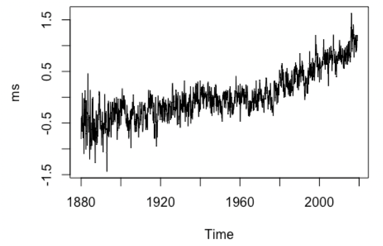
Because the series seems to be linearly increasing, to eliminate linearity we will difference once. Technically, the process can be looked at as an ARIMA(p, 1, q) model for the series. The plot of the differenced series shows stationary with consistent mean and variance throughout time.
plot(diff(ms), type='l')
diffms = diff(ms)
acf2(diffms)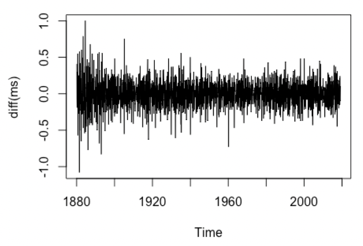
To help choose the values for the parameters, p and q, the plots of the acf and pacf will be observed.
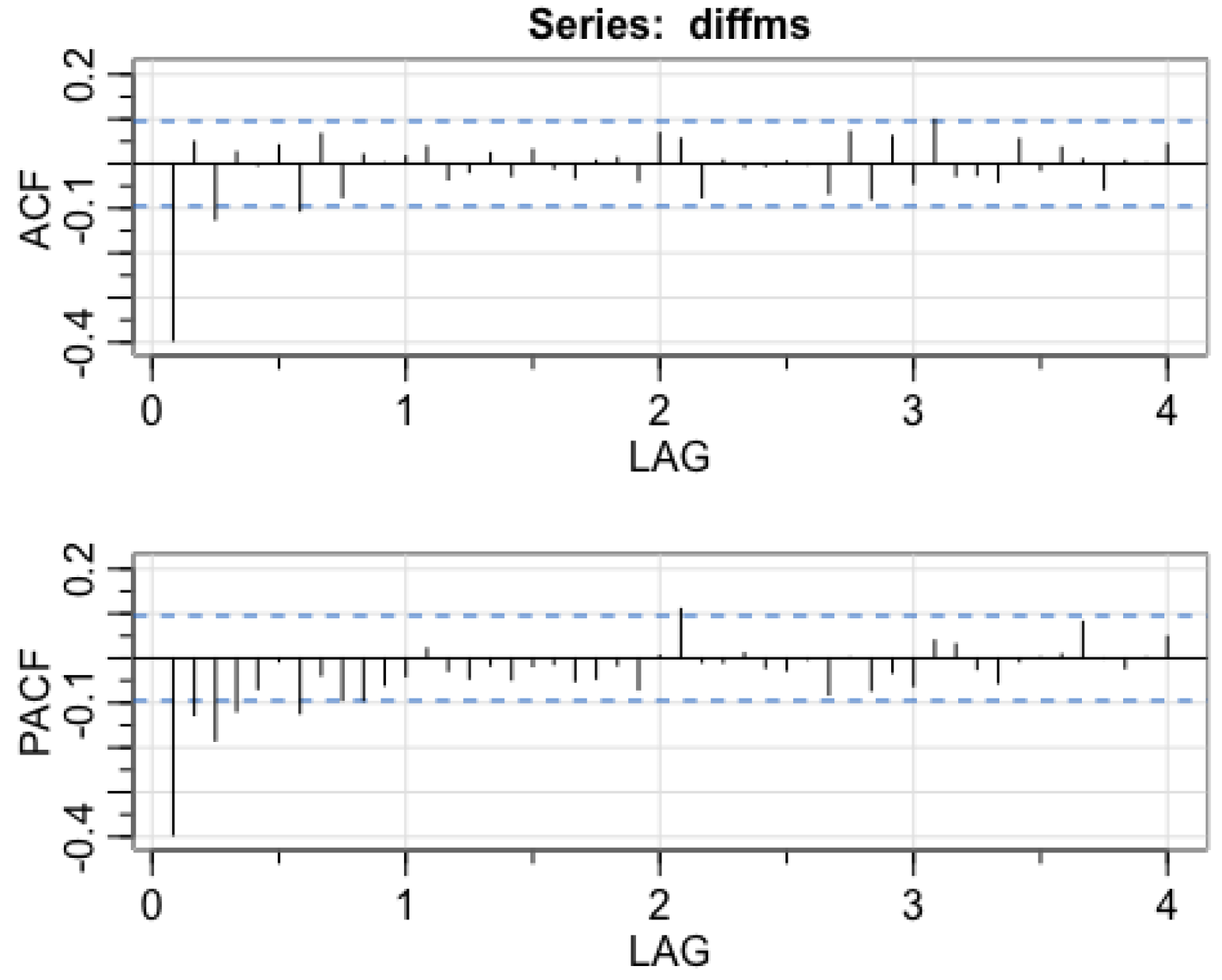
The significant lags of pure AutoRegressive (AR) models will cut off after lag p in the PACF function. While the significant lags of pure Moving Average (MA) models will cut off after lag q in the ACF function. The sample ACF and PACF look consistent with x being either an MA(1) process or an AR(8) process. The ARIMA process of the original undifferenced series corresponds to ARIMA(0,1,1) and ARIMA(8,1,0).
Since we are fitting the differenced data, the process used will be ARIMA(0,0,1) and ARIMA(8,0,0) respectively. We can also exclude the include.DRIFT=TRUE.
fitMA1 <- Arima(diffms, order=c(0,0,1), method='ML')
fitAR8 <- Arima(diffms, order=c(8,0,0), method='ML')

summary(fitMA1)

#=> prints Series: diffms
#=> ARIMA(0,0,1) with non-zero mean
##
## Coefficients:
##           ma1    mean
##       -0.5847  0.0010
## s.e.   0.0290  0.0018
##
## sigma^2 estimated as 0.03032:  log likelihood=549.94
## AIC=-1093.88   AICc=-1093.86   BIC=-1077.62
summary(fitAR8)
#=> prints Series: diffms
## ARIMA(8,0,0) with non-zero mean
## Coefficients:
##           ar1      ar2      ar3      ar4      ar5      ar6      ar7      ar8
##       -0.5223  -0.3403  -0.2770  -0.2586  -0.2340  -0.1897  -0.1492  -0.0557
## s.e.   0.0245   0.0274   0.0282   0.0285   0.0285   0.0282   0.0274   0.0246
##         mean
##       0.0010
## s.e.  0.0014
##
## sigma^2 estimated as 0.02923:  log likelihood=584.01
## AIC=-1148.02   AICc=-1147.89   BIC=-1093.82
We see that the fitted MA(1) model has σ=.03. The fitted AR(4) model has σ=.029. At this point, both models look similarly promising. To rule out one model, diagnostic plots will be observed to cancel the model with a bad fit.
sfitMA1 <- sarima(diffms, p=0, d=0, q=1)
sfitAR8 <- sarima(diffms, p=8, d=0, q=0)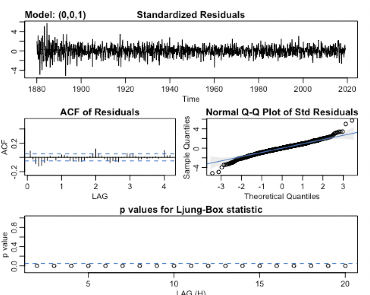
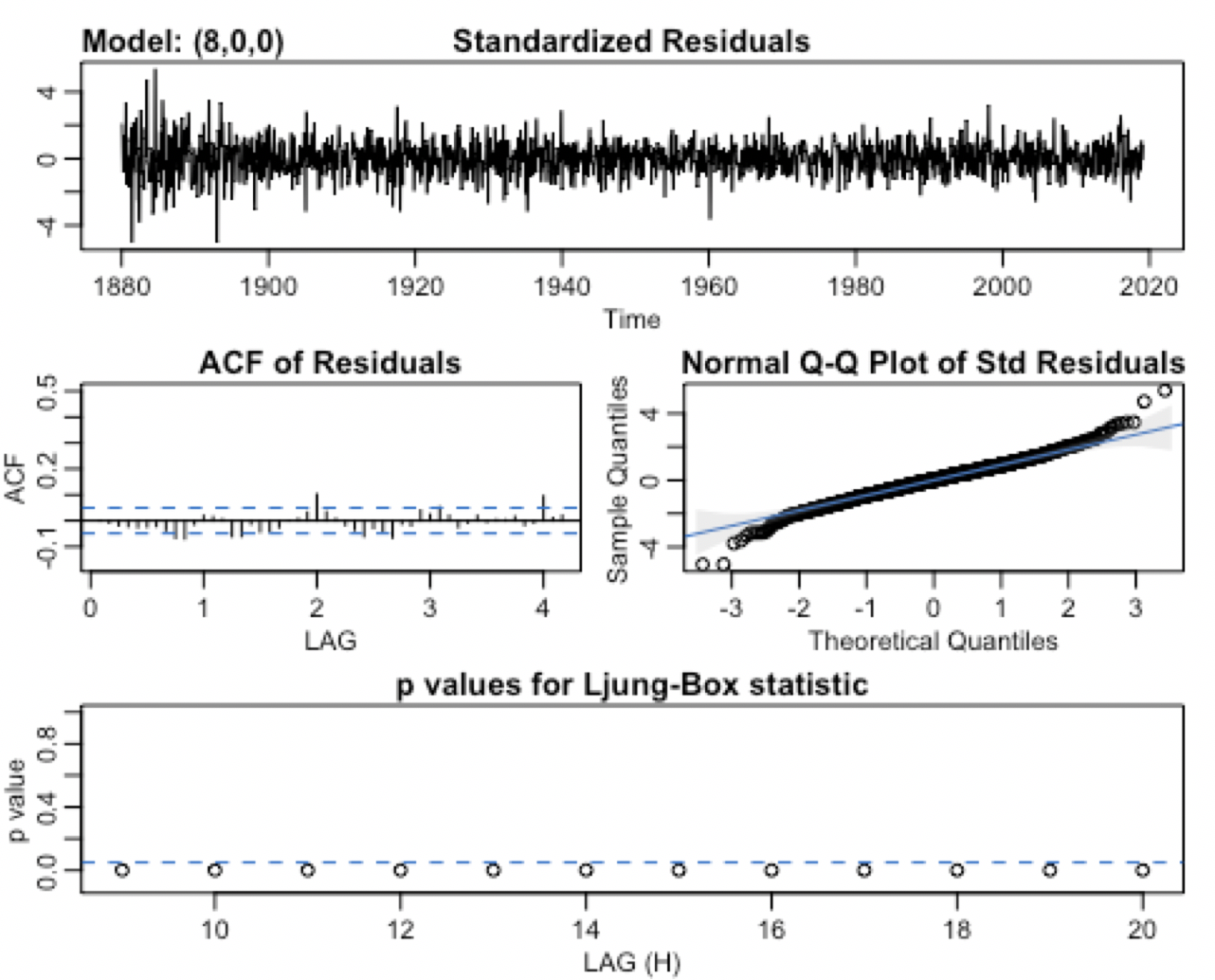 The diagnostic plots for both models seem to show that both models are promising. For the MA(1) model, the ACF of residuals show that six out of 25 lags are significant while the QQ points generally fit along the line. The tails of the plot stray away from the normal line. Similarly the AR(8) model only has about four out of 25 significant lags and a good fit of the normal QQ plot. Though the tail ends of the qq plot stray away from the normal line, the model still seems to be acceptable. The standardized results plot for both models show that the residuals closely mimic white noise and is stationary with constant mean and variance throughout.
Since there is not a model that I can rule out with the diagnostic plots, I will choose the model with the lowest Information Criteria Metrics (AICC, AIC, BIC) that penalizes model complexity and prediction error.
fitAR8$aic # Lowest
## [1] -1148.022
fitMA1$aic
## [1] -1093.876
fitAR8$aicc # Lowest
## [1] -1147.889
fitMA1$aicc
## [1] -1093.861
fitAR8$bic # Lowest
## [1] -1093.822
fitMA1$bic
## [1] -1077.616
All three information criteria results (aic,aicc,bic) show that AR(8) have the lowest error and is the better choice than MA(1).
By narrowing my model choice to only AR(8), I will forecast for the next 24 months which translates to 2 years from 2020 to 2022.
fitforecast <- Arima(ms, order=c(8,1,0),include.drift=TRUE)
fcAR8 <- forecast(fitforecast, h=24)
plot(fcAR8)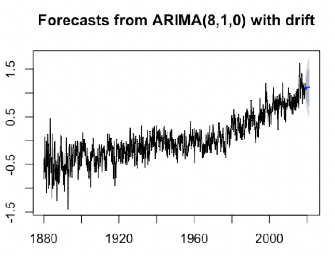
The blue line shows my line of prediction for the temperature deviation in the next two years. The shaded grey and blue lines show the .95 confidence interval of the prediction.